Robust fit
这一篇差不多是作为这个的后续
scipy.optimize.least_squares
用来搞Robust fit的有好几个,这里先从scipy的这个函数讲起
先看一下scipy cookbook里面的这个例子
这个例子里拟合了一个正弦函数
def generate_data(t, A, sigma, omega, noise=0, n_outliers=0, random_state=0):
    y = A * np.exp(-sigma * t) * np.sin(omega * t)
    rnd = np.random.RandomState(random_state)
    error = noise * rnd.randn(t.size)
    outliers = rnd.randint(0, t.size, n_outliers)
    error[outliers] *= 35
    return y + error
确定模型参数
A = 2
sigma = 0.1
omega = 0.1 * 2 * np.pi
x_true = np.array([A, sigma, omega])

noise = 0.1

t_min = 0
t_max = 30
将三个离群值放在fitting dataset里
t_train = np.linspace(t_min, t_max, 30)
y_train = generate_data(t_train, A, sigma, omega, noise=noise, n_outliers=4)
定义损失函数
def fun(x, t, y):
    return x[0] * np.exp(-x[1] * t) * np.sin(x[2] * t) - y
剩下就是一些常规的过程
x0 = np.ones(3)
from scipy.optimize import least_squares
res_lsq = least_squares(fun, x0, args=(t_train, y_train))
res_robust = least_squares(fun, x0, loss='soft_l1', f_scale=0.1, args=(t_train, y_train))
t_test = np.linspace(t_min, t_max, 300)
y_test = generate_data(t_test, A, sigma, omega)
y_lsq = generate_data(t_test, *res_lsq.x)
y_robust = generate_data(t_test, *res_robust.x)


plt.plot(t_train, y_train, 'o', label='data')
plt.plot(t_test, y_test, label='true')
plt.plot(t_test, y_lsq, label='lsq')
plt.plot(t_test, y_robust, label='robust lsq')
plt.xlabel('$t$')
plt.ylabel('$y$')
plt.legend();
很清楚的可以看出来,这里robust lsq结果明显更接近那个true的线
这里只用了soft l1,在least_squares里还有另外几个
loss str or callable, optional
Determines the loss function. The following keyword values are allowed:
- ‘linear’ (default) :
rho(z) = z. Gives a standard least-squares problem.- ‘soft_l1’ :
rho(z) = 2 * ((1 + z)**0.5 - 1). The smooth approximation of l1 (absolute value) loss. Usually a good choice for robust least squares.- ‘huber’ :
rho(z) = z if z <= 1 else 2*z**0.5 - 1. Works similarly to ‘soft_l1’.- ‘cauchy’ :
rho(z) = ln(1 + z). Severely weakens outliers influence, but may cause difficulties in optimization process.- ‘arctan’ :
rho(z) = arctan(z). Limits a maximum loss on a single residual, has properties similar to ‘cauchy’.
比较难受的就是这次没法像curve_fit那个函数一样那么好用了
就 我还要自己手动写个cost func
另一个例子
这个例子来自于这儿。
感谢这个例子教会我写cost func
Define the model function as y = a + b * exp(c * t), where t is a predictor variable, y is an observation and a, b, c are parameters to estimate
First, define the function which generates the data with noise and outliers, define the model parameters, and generate data:
>>> def gen_data(t, a, b, c, noise=0, n_outliers=0, random_state=0):
...     y = a + b * np.exp(t * c)
...
...     rnd = np.random.RandomState(random_state)
...     error = noise * rnd.randn(t.size)
...     outliers = rnd.randint(0, t.size, n_outliers)
...     error[outliers] *= 10
...
...     return y + error
...
>>> a = 0.5
>>> b = 2.0
>>> c = -1
>>> t_min = 0
>>> t_max = 10
>>> n_points = 15
...
>>> t_train = np.linspace(t_min, t_max, n_points)
>>> y_train = gen_data(t_train, a, b, c, noise=0.1, n_outliers=3)
Define function for computing residuals and initial estimate of parameters.
>>> def fun(x, t, y):
...     return x[0] + x[1] * np.exp(x[2] * t) - y
...
>>> x0 = np.array([1.0, 1.0, 0.0])NOTE: x0,x1,x2 corresponding to a,b,c; and t is what we always treat as x
Compute a standard least-squares solution:
>>> res_lsq = least_squares(fun, x0, args=(t_train, y_train))Now compute two solutions with two different robust loss functions. The parameter f_scale is set to 0.1, meaning that inlier residuals should not significantly exceed 0.1 (the noise level used).
>>> res_soft_l1 = least_squares(fun, x0, loss='soft_l1', f_scale=0.1,
...                             args=(t_train, y_train))
>>> res_log = least_squares(fun, x0, loss='cauchy', f_scale=0.1,
...                         args=(t_train, y_train))
t_test = np.linspace(t_min, t_max, n_points * 10)
>>> y_true = gen_data(t_test, a, b, c)
>>> y_lsq = gen_data(t_test, *res_lsq.x)
>>> y_soft_l1 = gen_data(t_test, *res_soft_l1.x)
>>> y_log = gen_data(t_test, *res_log.x)
...
>>> import matplotlib.pyplot as plt
>>> plt.plot(t_train, y_train, 'o')
>>> plt.plot(t_test, y_true, 'k', linewidth=2, label='true')
>>> plt.plot(t_test, y_lsq, label='linear loss')
>>> plt.plot(t_test, y_soft_l1, label='soft_l1 loss')
>>> plt.plot(t_test, y_log, label='cauchy loss')
>>> plt.xlabel("t")
>>> plt.ylabel("y")
>>> plt.legend()
>>> plt.show()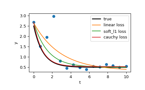
这个例子后面还有一个解决复数优化的问题,可真是牛逼
scikit learn
这个大体上相同,
from matplotlib import pyplot as plt
import numpy as np

from sklearn.linear_model import (
    LinearRegression, TheilSenRegressor, RANSACRegressor, HuberRegressor)
from sklearn.metrics import mean_squared_error
from sklearn.preprocessing import PolynomialFeatures
from sklearn.pipeline import make_pipeline

np.random.seed(42)

X = np.random.normal(size=400)
y = np.sin(X)
# Make sure that it X is 2D
X = X[:, np.newaxis]

X_test = np.random.normal(size=200)
y_test = np.sin(X_test)
X_test = X_test[:, np.newaxis]

y_errors = y.copy()
y_errors[::3] = 3

X_errors = X.copy()
X_errors[::3] = 3

y_errors_large = y.copy()
y_errors_large[::3] = 10

X_errors_large = X.copy()
X_errors_large[::3] = 10

estimators = [('OLS', LinearRegression()),
              ('Theil-Sen', TheilSenRegressor(random_state=42)),
              ('RANSAC', RANSACRegressor(random_state=42)),
              ('HuberRegressor', HuberRegressor())]
colors = {'OLS': 'turquoise', 'Theil-Sen': 'gold', 'RANSAC': 'lightgreen', 'HuberRegressor': 'black'}
linestyle = {'OLS': '-', 'Theil-Sen': '-.', 'RANSAC': '--', 'HuberRegressor': '--'}
lw = 3

x_plot = np.linspace(X.min(), X.max())
for title, this_X, this_y in [
        ('Modeling Errors Only', X, y),
        ('Corrupt X, Small Deviants', X_errors, y),
        ('Corrupt y, Small Deviants', X, y_errors),
        ('Corrupt X, Large Deviants', X_errors_large, y),
        ('Corrupt y, Large Deviants', X, y_errors_large)]:
    plt.figure(figsize=(5, 4))
    plt.plot(this_X[:, 0], this_y, 'b+')

    for name, estimator in estimators:
        model = make_pipeline(PolynomialFeatures(3), estimator)
        model.fit(this_X, this_y)
        mse = mean_squared_error(model.predict(X_test), y_test)
        y_plot = model.predict(x_plot[:, np.newaxis])
        plt.plot(x_plot, y_plot, color=colors[name], linestyle=linestyle[name],
                 linewidth=lw, label='%s: error = %.3f' % (name, mse))

    legend_title = 'Error of Mean\nAbsolute Deviation\nto Non-corrupt Data'
    legend = plt.legend(loc='upper right', frameon=False, title=legend_title,
                        prop=dict(size='x-small'))
    plt.xlim(-4, 10.2)
    plt.ylim(-2, 10.2)
    plt.title(title)
plt.show()
有个PolynomialFeatures(3)的意思是,可以从0阶多项式拟合到3阶多项式
Robust fitting is demoed in different situations:
- No measurement errors, only modelling errors (fitting a sine with a polynomial)
- Measurement errors in X
- Measurement errors in y
The median absolute deviation to non corrupt new data is used to judge the quality of the prediction.
What we can see that:
- RANSAC is good for strong outliers in the y direction
- TheilSen is good for small outliers, both in direction X and y, but has a break point above which it performs worse than OLS.
- The scores of HuberRegressor may not be compared directly to both TheilSen and RANSAC because it does not attempt to completely filter the outliers but lessen their effect.
iterative bi-square method
其实我最想找的是这个,这个来源于这篇文献
但是找来找去都没找到python的包
啊 又逼着我改用R了