Mixture Density Network (1)

2021-12-28 21 min

以前IOPの論文で述べたように、逆問題の数学的本質は不良設定問題です。機械学習とディープラーニングは本質的に分類と回帰問題を解決するもので、不良設定問題を直接解決することはできません。最近いくつかの論文を見直して、以前読んだことを思い出しました。

いくつかの論文

“Seamless retrievals of chlorophyll-a from Sentinel-2 (MSI) and Sentinel-3 (OLCI) in inland and coastal waters: A machine-learning approach”. N. Pahlevan, et al. (2020). Remote Sensing of Environment. 111604. 10.1016/j.rse.2019.111604.
“Robust algorithm for estimating total suspended solids (TSS) in inland and nearshore coastal waters”. S.V. Balasubramanian, et al. (2020). Remote Sensing of Environment. 111768. 10.1016/j.rse.2020.111768. Code.
“Hyperspectral retrievals of phytoplankton absorption and chlorophyll-a in inland and nearshore coastal waters”. N. Pahlevan, et al. (2021). Remote Sensing of Environment. 112200. 10.1016/j.rse.2020.112200.
“A Chlorophyll-a Algorithm for Landsat-8 Based on Mixture Density Networks”. B. Smith, et al. (2021). Frontiers in Remote Sensing. 623678. 10.3389/frsen.2020.623678.

これらの論文はすべてPahlevanによるもので、コードはhttps://github.com/BrandonSmithJ/MDNにありますが、盗まれるのを恐れているかのように、再適用方法については一切触れていません。

一つずつ見ていきましょう。

Seamless retrievals of chlorophyll-a from Sentinel-2 (MSI) and Sentinel-3 (OLCI) in inland and coastal waters: A machine-learning approach

これはPahlevanの最初の論文です。彼らのネットワークがどのように構築されているかに焦点を当てましょう。MDNの原理は後で実装と一緒に説明します。

訓練プロセス

データが十分にあったため、1/3のみ、約1000データポイントを訓練に使用しました。

入力データは400-800nmのRrsのみです。

すべての特徴量はlog変換され、中央値センタリングと四分位範囲スケーリングに基づいて正規化され、(0,1)の範囲にスケーリングされます。

このステップはどのように行われるのでしょうか？ソースコードを調べました。入力データに対して、from .transformers import TransformerPipeline, generate_scalersを使用して変換を行います。

そして：

from sklearn import preprocessing
args.x_scalers = [
			serialize(preprocessing.RobustScaler),
	]
	args.y_scalers = [
		serialize(LogTransformer),
		serialize(preprocessing.MinMaxScaler, [(-1, 1)]),
	]

あれ、0-1って言ってなかった？

具体的に使用されているのはhttps://scikit-learn.org/stable/modules/generated/sklearn.preprocessing.RobustScaler.htmlで、yにはMinMaxScalerを使用しています。

これらのパラメータを保存して後で再利用するはずです。そうでなければ単一の数値のIQRはどこから来るのでしょうか。

実際の実装時に詳しく見てみましょう。

出力データ：出力変数も同じ正規化方法が適用されます。

そしてこの図を載せています。

いや、特徴量エンジニアリングをどこでやったか見当たらないんですが。

後の論文を読んでいると、特徴量エンジニアリングの部分が削除されていることに気づきました（笑）。トップジャーナルでも問題が起きやすいですね。

ハイパーパラメータ調整について：

These choices appear to be fairly robust to changes within the current implementation, especially with regard to the MDN-specific parameters. Following experimenting with several architectures, we found that the model is very robust to changes in various hyperparameters.

この場合、彼らは5層のニューラルネットワークで各層100ニューロン、5つのガウス分布のパラメータを出力するように訓練しただけです。

ランダムなネットワーク初期化の10回の試行の中央値推定が、与えられたRrsスペクトルに対する予測Chlaです。すべての試行で同じ訓練データが使用されます。

この論文のネットワーク部分は基本的にこれで終わりです。次を見ましょう。

Robust algorithm for estimating total suspended solids (TSS) in inland and nearshore coastal waters

訓練プロセスに直接ジャンプします。

正直言って、こんなに直接的なコピペで、多くの部分が同じなのに、盗作と判定されないのでしょうか。この論文の面白いところは、MDN、QAA、水体光学分類を組み合わせてTSSを推定していることです。

前の論文との違いは：

The current default model uses a five-layer neural network with 25 neurons per layer, which is trained to output the parameters of five Gaussians. From this mixture model, the overall estimate is selected via the Gaussian with the maximum prior likelihood. The described model is trained a number of times with random initializations of the underlying neural network, in order to ensure a stable final output of the estimates. The median estimate is taken as the final result of these trials, with convergence occurring within some small margin of error after approximately ten trials

Hyperspectral retrievals of phytoplankton absorption and chlorophyll-a in inland and nearshore coastal waters

他に違いはありません。

強いて言えば、2つのモデルを訓練していますが、なぜ2つ必要なのかよくわかりません。

A Chlorophyll-a Algorithm for Landsat-8 Based on Mixture Density Networks

この論文はこう述べています：

All models examined in this study have simply used ‘reasonable’ default values for their hyperparameters (Glorot and Bengio 2010; Hinton 1990; Kingma and Ba 2014) namely: a five layer neural network with 100 nodes per layer, learning a mixture of five gaussians; a learning rate, L2 normalization rate, and value all set to 0.001; and with training performed via Adam optimization over a set of 10,000 stochastic mini-batch iterations, using a mini-batch size of 128 samples.

この論文は実際にとても興味深いです。

この論文の主な目的の一つは、逆問題専用に設計されたネットワークアーキテクチャであるMDNが、他のニューラルネットワークアーキテクチャと比較して優れていることを示すことです。具体的な結果はこれらの図を参照してください。

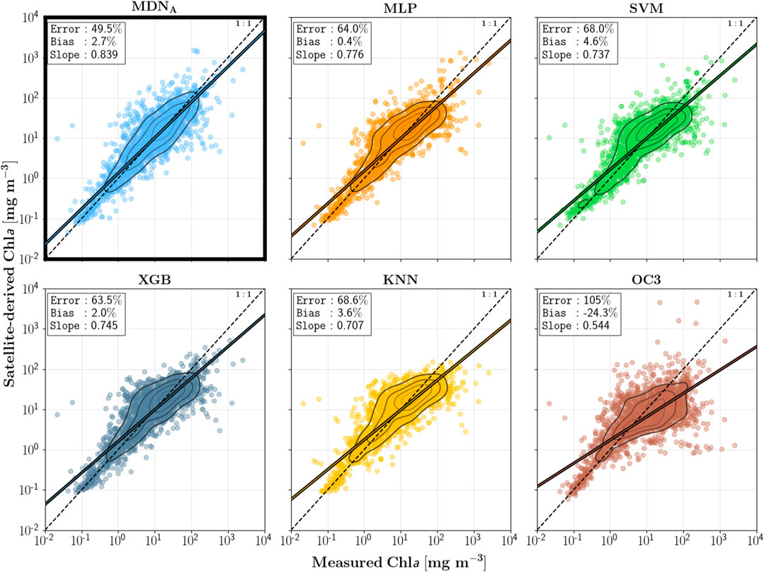
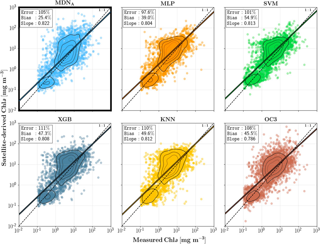
Cao 2020が使用し、私も試してみたかったXGBoostとも比較しています。

この論文の補足資料の議論も非常に興味深いです。この議論は特定の査読者に反論するために書かれたように感じます。この議論を翻訳してみましょう。

査読者の質問：なぜモデルのパラメータを調整しないのですか？

While no hyperparameter optimization has taken place over the course of this work, it is an important step to ensure optimal performance and generality.
These choices are mostly arbitrary, as the goal of this study was to present the feasibility and theoretical backing of the MDN model
These choices are mostly arbitrary, as the goal of this study was to present the feasibility and theoretical backing of the MDN model. A full optimality demonstration, on the other hand, would require a significantly longer study than already presented.

回答：第一に、それは焦点ではありません。第二に、時間がないので、まず論文を出しましょう。

査読者：ダメです、モデルパラメータが重要でないことを証明する必要があります。

Nevertheless, we would be remiss to exclude any discussion which examines the hyperparameter choices, and so what follows is a (very) brief look at how select parameters affect performance.

回答：わかりました、あなたが理解していないので、少し説明しましょう。そして、どうせ理解できないと思うので、最も簡単な部分を説明します。

First, some terminology must be defined in order to make it clear what is being examined. Normally in hyperparameter optimization, and machine learning in general, the dataset is split into three parts: training, validation, and testing. The training set is of course used to train the model on; the validation set is used to optimize the model using data unseen during training; and the testing set is used only at the end, in order to benchmark performance.

回答：定義を説明しましょう。

As mentioned, no explicit hyperparameter optimizations have taken place thus far in the study. Default values were chosen based on those commonly used in literature and in available libraries (e.g. scikit-learn), and as will be seen, do not represent the optimal values for our specific data. As such, no separate validation set was set aside for the purposes of such an exercise.

正確なハイパーパラメータ調整を行わなかったため、検証セットは作成せず、訓練とテストのみです。

One of the main questions any reader may have is, “how large is the model?”.

この分野の専門家ではないので専門的な質問ができないでしょうから、私が質問を提起しましょう。

そして、レイヤーとノードの影響を示す2つの図を示しました。

次に学習曲線を示しました。

査読者への反論が本当に上手いですね（笑）

ソースコードを読む前の知識補充

読みたくなければスキップしてください。

クラスに関する知識補充

以前サボった授業は別の形で戻ってきます。オブジェクト指向プログラミング、また来ました。

クラスには変数と関数の両方が含まれます。前者はクラスの属性、後者はクラスのメソッドです。

例えば、人の身長と体重は属性で、話すことや食べることはメソッドです。

定義方法：

class ClassName:
   'クラスのヘルプ情報'   # クラスドキュメント文字列
   class_suite  # クラス本体

# 例
class Employee:
   '全従業員の基底クラス'
   empCount = 0  # 属性

   def __init__(self, name, salary):
      self.name = name
      self.salary = salary
      Employee.empCount += 1

   def displayCount(self):  # メソッド
     print "Total Employee %d" % Employee.empCount

   def displayEmployee(self):
      print "Name : ", self.name,  ", Salary: ", self.salary

ここで、empCountはすべてのインスタンス間で共有されるクラス変数で、Employee.empCountでアクセスします。

最初のメソッド__init__()は、クラスのコンストラクタまたは初期化メソッドと呼ばれる特別なメソッドです。クラスのインスタンスが作成されると呼び出されます。つまり、クラスインスタンスを作成するたびに、nameとsalaryが割り当てられ、Employee.empCountが1増加します。

ここで、selfはインスタンスを表します。例えば「李華」を定義すると、selfは李華を表します。fun(x,y,z)を定義してfun(a,b,c)で呼び出すようなもので、selfは内部名にすぎず、呼び出し時に渡す必要はありません。

これがクラスと関数の特別な違いです。クラスには追加の最初のパラメータ名が必要です。

より具体的な違い：

class Test:
    def prt(self):
        print(self)
        print(self.__class__)
t = Test()
t.prt()

出力：

<__main__.Test instance at 0x10d066878>
__main__.Test

最初の行はインスタンスを出力し、2行目はクラス自体です。

selfはキーワードではありません。akb48に変更することもできます。

呼び出すにはインスタンスを作成する必要があります：

# "最初のEmployeeオブジェクトを作成"
emp1 = Employee("Zara", 2000)
# "2番目のEmployeeオブジェクトを作成"
emp2 = Employee("Manni", 5000)

これらのパラメータはinitを通じて受け取られます。

関数と同様に、インスタンス内の属性を変更およびアクセスできます：

emp1.displayEmployee()
emp2.displayEmployee()
print "Total Employee %d" % Employee.empCount

出力：

Name :  Zara ,Salary:  2000
Name :  Manni ,Salary:  5000
Total Employee 2

クラス属性の追加、削除、変更もできます：

emp1.age = 7  # 'age'属性を追加
emp1.age = 8  # 'age'属性を変更
del emp1.age  # 'age'属性を削除

これらの関数を使用して属性にアクセスすることもできます：

getattr(obj, name[, default])：オブジェクト属性にアクセス
hasattr(obj, name)：属性が存在するか確認
setattr(obj, name, value)：属性を設定。存在しない場合は新規作成
delattr(obj, name)：属性を削除

hasattr(emp1, 'age')    # 'age'が存在すればTrueを返す
getattr(emp1, 'age')    # 'age'の値を返す
setattr(emp1, 'age', 8) # 'age'属性を値8で追加
delattr(emp1, 'age')    # 'age'属性を削除

Pythonにはクラス作成時に存在する組み込みクラス属性があります：

dict：クラス属性（クラスデータ属性の辞書）
doc：クラスドキュメント文字列
name：クラス名
module：クラスが定義されているモジュール
bases：すべての親クラス（親クラスのタプル）

アクセス方法：

class Employee:
   '全従業員の基底クラス'
   empCount = 0

   def __init__(self, name, salary):
      self.name = name
      self.salary = salary
      Employee.empCount += 1

   def displayCount(self):
     print "Total Employee %d" % Employee.empCount

   def displayEmployee(self):
      print "Name : ", self.name,  ", Salary: ", self.salary

print "Employee.__doc__:", Employee.__doc__
print "Employee.__name__:", Employee.__name__
print "Employee.__module__:", Employee.__module__
print "Employee.__bases__:", Employee.__bases__
print "Employee.__dict__:", Employee.__dict__

出力：

Employee.__doc__: 全従業員の基底クラス
Employee.__name__: Employee
Employee.__module__: __main__
Employee.__bases__: ()
Employee.__dict__: {'__module__': '__main__', ...}

クラスの継承とポリモーフィズム

オブジェクト指向プログラミングの最大の利点はコードの再利用です。

コードで見た方が理解しやすいです：

class Parent:        # 親クラスを定義
   parentAttr = 100
   def __init__(self):
      print "親クラスのコンストラクタを呼び出し"

   def parentMethod(self):
      print '親クラスのメソッドを呼び出し'

   def setAttr(self, attr):
      Parent.parentAttr = attr

   def getAttr(self):
      print "親クラスの属性 :", Parent.parentAttr

class Child(Parent): # 子クラスを定義
   def __init__(self):
      print "子クラスのコンストラクタを呼び出し"

   def childMethod(self):
      print '子クラスのメソッドを呼び出し'

c = Child()          # 子クラスをインスタンス化
c.childMethod()      # 子クラスのメソッドを呼び出し
c.parentMethod()     # 親クラスのメソッドを呼び出し
c.setAttr(200)       # 親クラスのメソッドを再度呼び出し
c.getAttr()          # 親クラスのメソッドを再度呼び出し

親クラスは最も基本的な属性とメソッドのみを定義します。

ポリモーフィズムは、例えばEmployeeにこのメソッドを追加するようなものです：

class Employee:
   def print_title(self):
        if self.sex == "male":
            print("man")
        elif self.sex == "female":
            print("woman")

今、児童労働者を雇いたい場合、新しいサブクラスを書けます：

class child(Employee):
     def print_title(self):
        if self.sex == "male":
             print("boy")
         elif self.sex == "female":
             print("girl")

子クラスと親クラスの両方に同じprint_title()メソッドがある場合、子クラスのprint_title()が親クラスのものをオーバーライドします。実行時には子クラスのprint_title()が呼び出されます。

ポリモーフィズムの利点は、Teenagers、Grownupsなどのサブクラスが必要な場合、Personを継承するだけでよいことです。これが「オープン・クローズド」原則です。

イテレータ

どのようなクラスがループできるかについて - 今のところ必要ないと思います。

アクセス制限

属性を外部からアクセスさせたくない場合、アクセス制限を追加できます：

class JustCounter:
	__secretCount = 0  # プライベート変数
	publicCount = 0    # パブリック変数

	def count(self):
		self.__secretCount += 1
		self.publicCount += 1
		print self.__secretCount

counter = JustCounter()
counter.count()
counter.count()
print counter.publicCount
print counter.__secretCount  # エラー、インスタンスはプライベート変数にアクセスできない

モジュールのインポート

Pythonモジュールは.pyで終わるPythonファイルで、Pythonオブジェクト定義とステートメントを含みます。

つまり、クラスをモジュールに入れて、関数のように呼び出すことができます。

MDNの実装

ここまで説明しましたが、MDNとは何でしょうか？

これと一緒に説明する予定です。

MDNがどのように実装されているかに焦点を当て、論文のソースコードと比較します。最後に原理を説明します。

これを読む前に、まずこのチュートリアルを完了してください。

class MDN(nn.Module):
    def __init__(self, n_hidden, n_gaussians):
        super(MDN, self).__init__()
        self.z_h = nn.Sequential(  # 連続処理：線形変換後にtanh
            nn.Linear(1, n_hidden),  # ここで線形変換
            nn.Tanh()
        )
        self.z_pi = nn.Linear(n_hidden, n_gaussians)
        self.z_sigma = nn.Linear(n_hidden, n_gaussians)
        self.z_mu = nn.Linear(n_hidden, n_gaussians)
    def forward(self, x):
        z_h = self.z_h(x)
        pi = nn.functional.softmax(self.z_pi(z_h), -1)
        # [0,1]にリスケール
        sigma = torch.exp(self.z_sigma(z_h))
        # exp演算
        mu = self.z_mu(z_h)
        return pi, sigma, mu

このMDNがどのように構築されているか詳しく説明しましょう。

各入力xに対して、yの分布を予測します：

$P(y|x) = \sum_{k}^{K} \Pi_{k}(x) \phi(y, \mu_{k}(x), \sigma_{k}(x))$

$k$ は参照しているガウス分布のインデックス。合計 $K$ 個のガウス分布があります。
$\sum_{k}^{K}$ は総和演算子。すべての $K$ にわたって各 $k$ ガウス分布を合計します。
$\Pi_k$ は各 $k$ ガウス分布を混合するための重みまたは乗数として機能します。入力 $x$ の関数です： $\Pi_k(x)$
$\phi$ はガウス関数で、与えられた平均と標準偏差に対する $y$ での値を返します。
$\mu_k$ と $\sigma_k$ は $k$ ガウス分布のパラメータ：平均 $\mu_k$ と標準偏差 $\sigma_k$ 。各ガウス分布で固定ではなく、入力 $x$ の関数でもあります。

すべての $\sigma_{k}$ は正で、すべての重み $\Pi$ の合計は1です：

$\sum_{k}^{K} \Pi_{k} = 1$

まず、ネットワークは各 $k$ ガウス分布に対して関数 $\Pi_{k}(x), \mu_{k}(x), \sigma_{k}(x)$ を学習する必要があります。これらの関数を使用して、与えられた入力 $x$ に対する個々のパラメータ $\mu_k, \sigma_k, \Pi_k$ を生成できます。

実装では、20ノードの1つの隠れ層を持つニューラルネットワークを使用します。これは5つの混合のパラメータを生成する別の層に供給されます。

定義は3つの部分に分かれます。

まず、入力 $x$ から20個の隠れ値 $z_h$ を計算します。

$z_h(x) = \tanh( W_{in} x + b_{in})$

次に、これらの隠れ値 $z_h$ を使用して3セットのパラメータ $\Pi, \sigma, \mu$ を計算します：

$z_\Pi = W_{\Pi} z_h + b_{\Pi}\\ z_\sigma = W_{\sigma} z_h + b_{\sigma}\\ z_\mu = W_{\mu} z_h + b_{\mu}$

3番目に、これらの層の出力を使用してガウス分布のパラメータを決定します。

$\Pi = \frac{\exp(z_{\Pi})}{\sum_{k}^{K} \exp(z_{\Pi_k})}\\ \sigma = \exp(z_{\sigma})\\ \mu = z_{\mu}$

$\exp(x)$ は指数関数で、 $e^x$ とも書きます

softmax演算子を使用して、 $\Pi$ がすべての $k$ にわたって1になるようにし、指数関数は各重み $\Pi_k$ が正であることを保証します。また、指数関数を使用してすべての $\sigma_k$ が正であることを保証します。

わかりました。この構築方法は、MDNがガウス混合モデルのいくつかのパラメータを予測し、PDF全体から値を取って予測値とするものです。

これは一つの問題につながります：私のy値は1つの数値だけですが、MDNは分布を生成します。重みを更新するためのlossをどのように計算するのでしょうか？

次の記事をご覧ください。

Machine Learning Inversion Deep Learning