Scipy optimize

2021-01-01 8 min

Table of Contents

This article mainly covers several commonly used functions:

minimize

Least_square

nnls

Lsq_linear

Curve_fit

Additionally, there’s numpy.linalg.lstsq

Also, I discovered something quite tricky - generally x needs to be the first parameter of the function for fitting to work properly.

minimize

This is mainly used to replace fminunc in MATLAB.

scipy.optimize.minimize(fun, x0, args=(), method=None, jac=None, hess=None, hessp=None, bounds=None, constraints=(), tol=None, callback=None, options=None)

fun is the cost function to be minimized. The requirements for the cost function are:

fun
The objective function to be minimized.
fun(x, *args) -> float
where x is an 1-D array with shape (n,) and args is a tuple of the fixed parameters needed to completely specify the function.

x0 is the initial parameter, commonly known as the initial guess. Array of real elements of size (n,), where ‘n’ is the number of independent variables.

method: This parameter represents the method to use. The default is one of BFGS, L-BFGS-B, SLSQP, with TNC as an option.

jac is the method for computing gradients, which can be ignored most of the time. This is the Jacobian matrix.

options: Used to control the maximum number of iterations, set in dictionary form, for example: options={‘maxiter’

}

boundssequence or Bounds, optional
Bounds on variables for L-BFGS-B, TNC, SLSQP, Powell, and trust-constr methods. There are two ways to specify the bounds:
Instance of Bounds class.
Sequence of (min, max) pairs for each element in x. None is used to specify no bound.
constraints{Constraint, dict} or List of {Constraint, dict}, optional
Constraints definition (only for COBYLA, SLSQP and trust-constr).
Constraints for ‘trust-constr’ are defined as a single object or a list of objects specifying constraints to the optimization problem. Available constraints are:
LinearConstraint
NonlinearConstraint

bounds is mainly used to control upper and lower limits, while constraints narrows the range through relationships between variables.

tol: float, optional
Tolerance for termination. For detailed control, use solver-specific options.

tol is the minimum iteration value, which is the condition for stopping iteration.

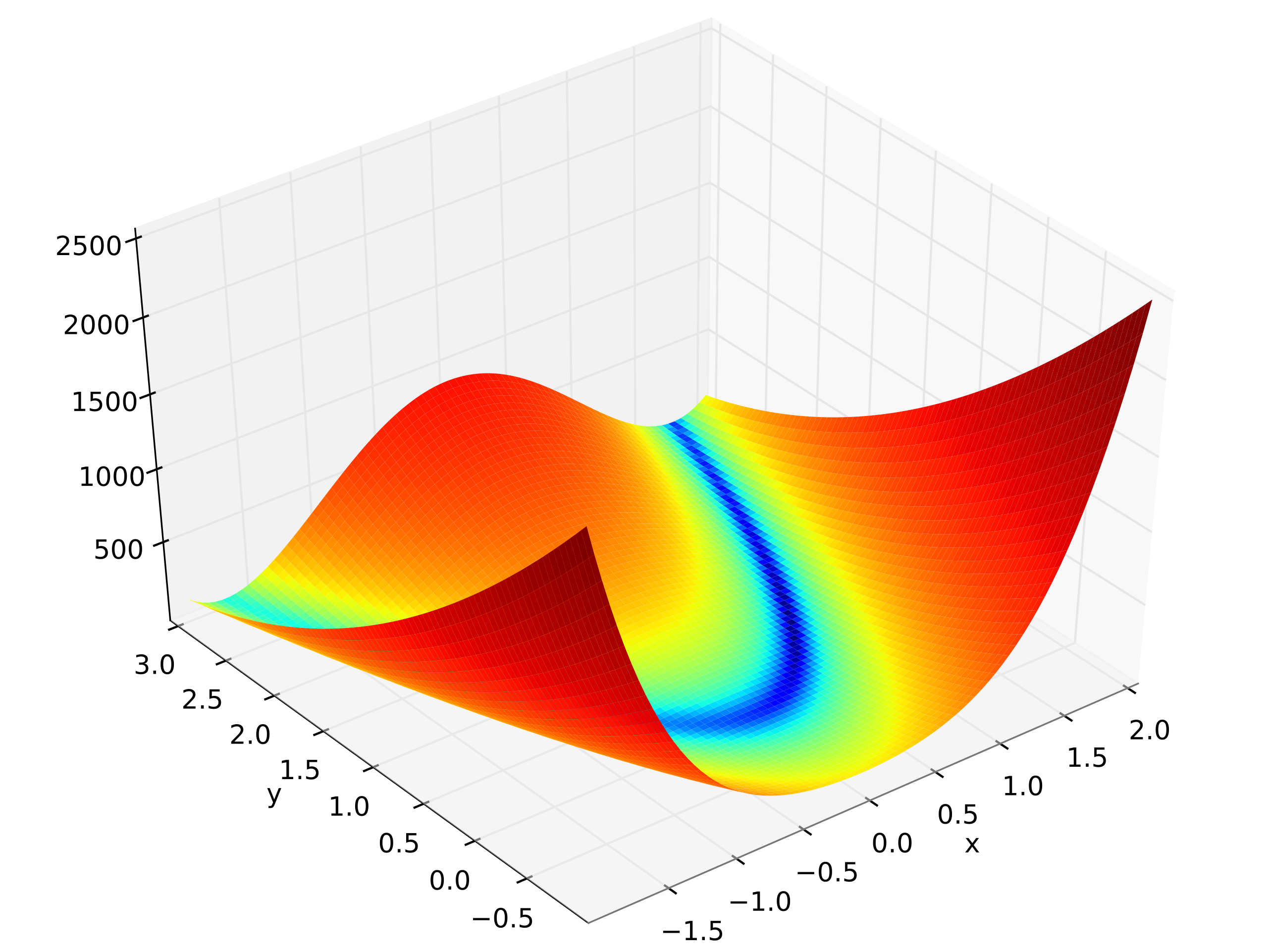
Here is the example of Rosenbrock function

f(x)=\sum_{i=1}^{N-1}100(x_{x+1}-x_i^2)+(1-x_i)^2

import numpy as np
from scipy.optimize import minimize

def rosen(x):
    """The Rosenbrock function"""
    return sum(100.0*(x[1:]-x[:-1]**2.0)**2.0 + (1-x[:-1])**2.0)

x0 = np.array([1.3, 0.7, 0.8, 1.9, 1.2])
res = minimize(rosen, x0, method='nelder-mead',
               options={'xatol': 1e-8, 'disp': True})
Optimization terminated successfully.
         Current function value: 0.000000
         Iterations: 339
         Function evaluations: 571
>>>
print(res.x)
[1. 1. 1. 1. 1.]

More often, we need to use the boundaries or constraints. Here I show the boundary.

Least_square

scipy.optimize.least_squares(fun, x0, jac='2-point', bounds=- inf, inf, method='trf', ftol=1e-08, xtol=1e-08, gtol=1e-08, x_scale=1.0, loss='linear', f_scale=1.0, diff_step=None, tr_solver=None, tr_options={}, jac_sparsity=None, max_nfev=None, verbose=0, args=(), kwargs={})

This is almost the same as the previous one.

nnls

scipy.optimize.nnls(A, b, maxiter=None)

Solve argmin_x || Ax - b ||_2 for x>=0.

Parameters

**A **ndarray
Matrix A as shown above.
**b ** ndarray
Right-hand side vector.
maxiter: int, optional
Maximum number of iterations, optional. Default is 3 * A.shape[1].

Returns

**x ** ndarray
Solution vector.
**rnorm: float
The residual, || Ax-b ||_2.

lsq_linear

scipy.optimize.lsq_linear(A, b, bounds=- inf, inf, method='trf', tol=1e-10, lsq_solver=None, lsmr_tol=None, max_iter=None, verbose=0)

Solve a linear least-squares problem with bounds on the variables.

Given a m-by-n design matrix A and a target vector b with m elements, lsq_linear solves the following optimization problem:

minimize 0.5 * ||A x - b||**2
subject to lb <= x <= ub

curve_fit

scipy.optimize.curve_fit(f, xdata, ydata, p0=None, sigma=None, absolute_sigma=False, check_finite=True, bounds=- inf, inf, method=None, jac=None, **kwargs)

This is actually the most commonly used function.

Note that f here is not the cost function, but the model function, for example:

def f_1(x, A, B):
    return A * x + B

**xdata array_like or object **The independent variable where the data is measured. Should usually be an M-length sequence or an (k,M)-shaped array for functions with k predictors, but can actually be any object. Simply put, this is the array of independent variables to fit.
**ydata array_like **The dependent data, a length M array - nominallyf(xdata,...). Simply put, this is the array of dependent variable values to fit.
p0 array_like , optionalInitial guess for the parameters (length N). If None, then the initial values will all be 1 (if the number of parameters for the function can be determined using introspection, otherwise a ValueError is raised). This sets an initial value for your function’s parameters to reduce computational load.
Method to use for optimization. See least_squares for more details. Default is ‘lm’ for unconstrained problems and ‘trf’ if bounds are provided. The method ‘lm’ won’t work when the number of observations is less than the number of variables, use ‘trf’ or ‘dogbox’ in this case.

Here is the official example:

import matplotlib.pyplot as plt
from scipy.optimize import curve_fit

def func(x, a, b, c):
    return a * np.exp(-b * x) + c

Define the data to be fit with some noise:

xdata = np.linspace(0, 4, 50)
y = func(xdata, 2.5, 1.3, 0.5)
np.random.seed(1729)
y_noise = 0.2 * np.random.normal(size=xdata.size)
ydata = y + y_noise
plt.plot(xdata, ydata, 'b-', label='data'

Fit for the parameters a, b, c of the function func:

popt, pcov = curve_fit(func, xdata, ydata)
popt

plt.plot(xdata, func(xdata, *popt), 'r-',
         label='fit: a=%5.3f, b=%5.3f, c=%5.3f' % tuple(popt))

Constrain the optimization to the region of 0 <= a <= 3, 0 <= b <= 1 and 0 <= c <= 0.5:

popt, pcov = curve_fit(func, xdata, ydata, bounds=(0, [3., 1., 0.5]))
popt

plt.plot(xdata, func(xdata, *popt), 'g--',
         label='fit: a=%5.3f, b=%5.3f, c=%5.3f' % tuple(popt))

plt.xlabel('x')
plt.ylabel('y')
plt.legend()
plt.show()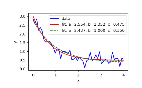

But there’s a question here: what if I want to fix the value of a, or I want to get a series of functions where each function has a fixed value of a?

In this case, you need to not treat a as a variable, and create another function to pass a in, for example:

custom_gaussian = lambda x, mu: gaussian(x, mu, 0.05)

Using lambda to create a small anonymous function:

import matplotlib.pyplot as plt
import numpy as np
import scipy.optimize

def gaussian(x, mu, sigma):
    return 1 / sigma / np.sqrt(2 * np.pi) * np.exp(-(x - mu)**2 / 2 / sigma**2)
# This is the original, full parameter gaussian function
# Create sample data
x = np.linspace(0, 2, 200)
y = gaussian(x, 1, 0.1) + np.random.rand(*x.shape) - 0.5
plt.plot(x, y, label="sample data")

# Fit with original fit function
popt, _ = scipy.optimize.curve_fit(gaussian, x, y)
plt.plot(x, gaussian(x, *popt), label="gaussian")

# Fit with custom fit function with fixed `sigma`
custom_gaussian = lambda x, mu: gaussian(x, mu, 0.05)
# this is the customized gaussian function that we want to fit
popt, _ = scipy.optimize.curve_fit(custom_gaussian, x, y)
plt.plot(x, custom_gaussian(x, *popt), label="custom_gaussian")

plt.legend()
plt.show()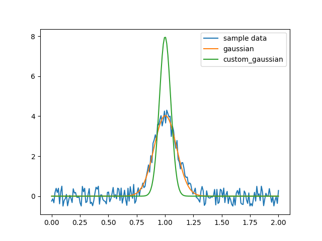

numpy.linalg.lstsq

This is numpy’s built-in least-squares solution to a linear matrix equation.

Here we need to recall the problem of systems of linear equations:

\begin{equation} \left\{ a_{1,1}x_1+a_{1,2}x_2+\cdots+a_{1,n}=b_1,\\ a_{2,1}x_1+a_{2,2}x_2+\cdots+a_{1,n}=b_2, \\ \vdots \\ a_{m,1}x_1+a_{m,2}x_2+...+a_{m,n}=b_m, \right. \end{equation}

(The formatting of this brace might have some issues)

Where $a_{1,1},\,a_{1,2}$ and $b_{1},\,b_{2}$ etc. are known constants, while $x_{1},\,x_{2}$ etc. are the unknowns to be solved.

Using linear algebra concepts, a system of linear equations can be written as:

Ax=b

A= \begin{bmatrix} a_{1,1}&\ a_{1,2}&\ \cdots&\ a_{1,n}\\ a_{2,1}&\ a_{2,2}&\ \cdots&\ a_{2,n}\\ \vdots&\ \vdots&\ \ddots&\ \vdots \\ a_{m,1}&\ a_{m,2}&\ \cdots&\ a_{m,n} \end{bmatrix} , \ x= \begin{bmatrix} x_{1}\\ x_{2}\\ \vdots\\ x_n \end{bmatrix} , b= \begin{bmatrix} b_{1}\\ b_{2}\\ \vdots\\ b_m \end{bmatrix}

Here A is an m×n matrix, x is a column vector with n elements, and b is a column vector with m elements.

If there is a set of numbers x1, x2, …xn that makes all the equations hold, then this set of numbers is called the solution of the system. The set of all solutions of a linear system is called the solution set. Based on the existence of solutions, linear systems can be classified into three types:

Exactly determined systems with a unique solution,
Overdetermined systems where no solution exists,
Underdetermined systems with infinitely many solutions (also commonly called indeterminate systems).
Linear algebra basically covers two things: how to determine if a solution exists and how to find the solution.
For a review of linear systems, see Linear Equations PDF

Loosely speaking, when m>n there is generally no solution, which is called an overdetermined system. However, in this case, the problem can be transformed into an optimization problem: find a set of x that minimizes $|Ax-b|^2$ . This is a least squares problem.

Parameters

a(M, N) array_like
“Coefficient” matrix.
b{(M,), (M, K)} array_like
Ordinate or “dependent variable” values. If b is two-dimensional, the least-squares solution is calculated for each of the K columns of b.
rcondfloat, optional
Cut-off ratio for small singular values of a. For the purposes of rank determination, singular values are treated as zero if they are smaller than rcond times the largest singular value of a.

Returns

x{(N,), (N, K)} ndarray
Least-squares solution. If b is two-dimensional, the solutions are in the K columns of x.
residuals{(1,), (K,), (0,)} ndarray
Sums of residuals; squared Euclidean 2-norm for each column in b - a*x. If the rank of a is < N or M <= N, this is an empty array. If b is 1-dimensional, this is a (1,) shape array. Otherwise the shape is (K,).
rankint
Rank of matrix a.

s(min(M, N),) ndarray

Singular values of a.

Examples for $y=mx+c$

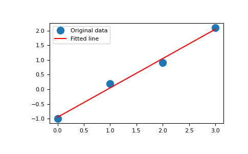
x = np.array([0, 1, 2, 3])
y = np.array([-1, 0.2, 0.9, 2.1])

By examining the coefficients, we see that the line should have a gradient of roughly 1 and cut the y-axis at, more or less, -1.

We can rewrite the line equation as y = Ap, where A = [[x 1]] and p = [[m], [c]]. Now use lstsq to solve for p:

A = np.vstack([x, np.ones(len(x))]).T
>>> A
array([[ 0.,  1.],
       [ 1.,  1.],
       [ 2.,  1.],
       [ 3.,  1.]])

m, c = np.linalg.lstsq(A, y, rcond=None)[0]
>>> m, c
(1.0 -0.95) # may vary

import matplotlib.pyplot as plt
>>> _ = plt.plot(x, y, 'o', label='Original data', markersize=10)
>>> _ = plt.plot(x, m*x + c, 'r', label='Fitted line')
>>> _ = plt.legend()
>>> plt.show()

Research python