Python Plotting Basics

2020-08-21 7 min

These past two days I’ve been organizing my plotting work and realized my matplotlib skills are really lacking. This note is to organize the things I’ll use, except for cartopy.

matplotlib

Basic Concepts

The most important basic concepts in Matplotlib are figure and axes.

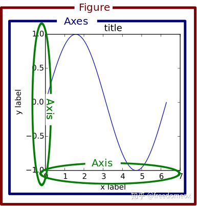
In Matplotlib, figure means the drawing board, axes means the canvas, and axis means the coordinate axis. For example:

x = np.linspace(0, 10, 20)  # Generate data
y = x * x + 2

fig = plt.figure()  # Create new figure object
axes = fig.add_axes([0.5, 0.5, 0.8, 0.8])  # Control canvas left, bottom, width, height
axes.plot(x, y, 'r')

On the same drawing board, we can draw multiple canvases:

fig = plt.figure()  # Create new drawing board
axes1 = fig.add_axes([0.1, 0.1, 0.8, 0.8])  # Large canvas
axes2 = fig.add_axes([0.2, 0.5, 0.4, 0.3])  # Small canvas

axes1.plot(x, y, 'r')  # Large canvas
axes2.plot(y, x, 'g')  # Small canvas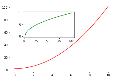

Additionally, there’s another way to add canvases using plt.subplots():

fig, axes = plt.subplots(nrows=1, ncols=2)  # Subplots: 1 row, 2 columns
for ax in axes:
    ax.plot(x, y, 'r')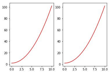

Even when drawing just one canvas, it’s recommended to use fig, axes = plt.subplots() to generate the canvas and drawing board for easier adjustment, rather than using plt.plot().

Basic Style Adjustments

Adding Title and Legend

Drawing a figure with title, axis labels, and legend:

fig, axes = plt.subplots()

axes.set_xlabel('x label')  # X-axis label
axes.set_ylabel('y label')
axes.set_title('title')  # Figure title

axes.plot(x, x**2)
axes.plot(x, x**3)
axes.legend(["y = x**2", "y = x**3"], loc=0)  # Legend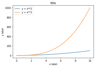

The loc parameter in legend marks the legend position. 1, 2, 3, 4 represent: top-right, top-left, bottom-left, bottom-right respectively; 0 means auto-adaptive.

Line Style, Color, Transparency

In Matplotlib, you can set line color, transparency, and other properties.

fig, axes = plt.subplots()

axes.plot(x, x+1, color="red", alpha=0.5)
axes.plot(x, x+2, color="#1155dd")
axes.plot(x, x+3, color="#15cc55")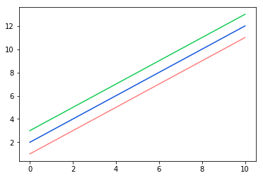

For line styles, besides solid and dashed lines, there are many rich line styles to choose from.

fig, ax = plt.subplots(figsize=(12, 6))

# Line width
ax.plot(x, x+1, color="blue", linewidth=0.25)
ax.plot(x, x+2, color="blue", linewidth=0.50)
ax.plot(x, x+3, color="blue", linewidth=1.00)
ax.plot(x, x+4, color="blue", linewidth=2.00)

# Dash types
ax.plot(x, x+5, color="red", lw=2, linestyle='-')
ax.plot(x, x+6, color="red", lw=2, ls='-.')
ax.plot(x, x+7, color="red", lw=2, ls=':')

# Dash spacing
line, = ax.plot(x, x+8, color="black", lw=1.50)
line.set_dashes([5, 10, 15, 10])

# Markers
ax.plot(x, x + 9, color="green", lw=2, ls='--', marker='+')
ax.plot(x, x+10, color="green", lw=2, ls='--', marker='o')
ax.plot(x, x+11, color="green", lw=2, ls='--', marker='s')
ax.plot(x, x+12, color="green", lw=2, ls='--', marker='1')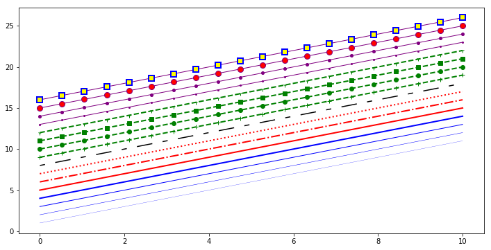

Canvas Grid, Axis Range

Sometimes we may need to display canvas grid or adjust axis range.

fig, axes = plt.subplots(1, 2, figsize=(10, 5))

# Show grid
axes[0].plot(x, x**2, x, x**3, lw=2)
axes[0].grid(True)

# Set axis range
axes[1].plot(x, x**2, x, x**3)
axes[1].set_ylim([0, 60])
axes[1].set_xlim([2, 5])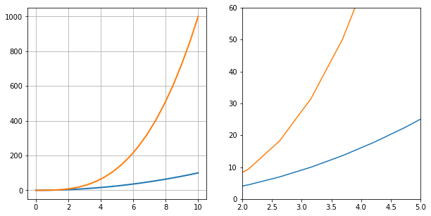

Besides line plots, Matplotlib also supports scatter plots, bar charts, and other common charts.

n = np.array([0, 1, 2, 3, 4, 5])

fig, axes = plt.subplots(1, 4, figsize=(16, 5))

axes[0].scatter(x, x + 0.25*np.random.randn(len(x)))
axes[0].set_title("scatter")

axes[1].step(n, n**2, lw=2)
axes[1].set_title("step")

axes[2].bar(n, n**2, align="center", width=0.5, alpha=0.5)
axes[2].set_title("bar")

axes[3].fill_between(x, x**2, x**3, color="green", alpha=0.5)
axes[3].set_title("fill_between")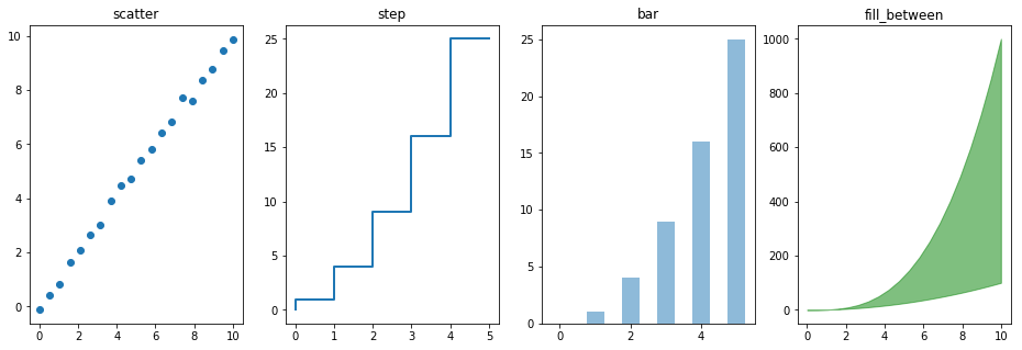

Figure Annotation Methods

When drawing complex images, annotations often have a finishing touch effect. Figure annotation means adding text notes, arrows, boxes, and other annotation elements to the image.

In Matplotlib, text annotation is implemented by matplotlib.pyplot.text(). The basic format is matplotlib.pyplot.text(x, y, s), where x, y are for positioning and s is the annotation string.

fig, axes = plt.subplots()

x_bar = [10, 20, 30, 40, 50]  # Bar chart x-coordinates
y_bar = [0.5, 0.6, 0.3, 0.4, 0.8]  # Bar chart y-coordinates
bars = axes.bar(x_bar, y_bar, color='blue', label=x_bar, width=2)
for i, rect in enumerate(bars):
    x_text = rect.get_x()  # Get bar x-coordinate
    y_text = rect.get_height() + 0.01  # Get bar height and add 0.01
    plt.text(x_text, y_text, '%.1f' % y_bar[i])  # Annotate text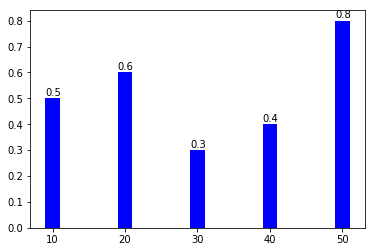

Besides text annotation, you can add arrow annotations using matplotlib.pyplot.annotate().

fig, axes = plt.subplots()

bars = axes.bar(x_bar, y_bar, color='blue', label=x_bar, width=2)
for i, rect in enumerate(bars):
    x_text = rect.get_x()
    y_text = rect.get_height() + 0.01
    plt.text(x_text, y_text, '%.1f' % y_bar[i])

    # Add arrow annotation
    plt.annotate('Min', xy=(32, 0.3), xytext=(36, 0.3),
                 arrowprops=dict(facecolor='black', width=1, headwidth=7))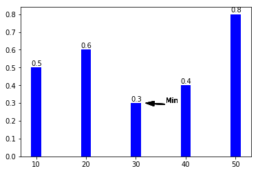

In the example above, xy=() represents the annotation endpoint coordinates, xytext=() represents the annotation start coordinates. For arrow drawing, arrowprops=() sets arrow style, facecolor= sets color, width= sets arrow tail width, headwidth= sets arrow head width.

Cheatsheet

Matplotlib officially provides cheatsheets, recommended to print and post in a visible place:

https://github.com/matplotlib/cheatsheets

3D Graphics

Basic 3D Graphics

Matplotlib can also draw 3D graphics. Unlike 2D graphics, 3D graphics are mainly implemented through the mplot3d module.

The mplot3d module mainly contains 4 major classes:

mpl_toolkits.mplot3d.axes3d()
mpl_toolkits.mplot3d.axis3d()
mpl_toolkits.mplot3d.art3d()
mpl_toolkits.mplot3d.proj3d()

First, let’s draw a 3D scatter plot:

import numpy as np
from mpl_toolkits.mplot3d import Axes3D
import matplotlib.pyplot as plt
%matplotlib inline

# x, y, z are 100 random numbers between 0 and 1
x = np.random.normal(0, 1, 100)
y = np.random.normal(0, 1, 100)
z = np.random.normal(0, 1, 100)

fig = plt.figure()

ax = Axes3D(fig)
ax.scatter(x, y, z)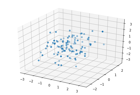

Line plots are similar to scatter plots, requiring x, y, z coordinate values:

# Generate data
x = np.linspace(-6 * np.pi, 6 * np.pi, 1000)
y = np.sin(x)
z = np.cos(x)

# Create 3D figure object
fig = plt.figure()
ax = Axes3D(fig)
ax.plot(x, y, z)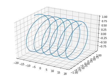

3D bar chart:

# Create 3D figure object
fig = plt.figure()
ax = Axes3D(fig)

# Generate data and plot
x = [0, 1, 2, 3, 4, 5, 6]
for i in x:
    y = [0, 1, 2, 3, 4, 5, 6, 7, 8, 9]
    z = abs(np.random.normal(1, 10, 10))
    ax.bar(y, z, i, zdir='y', color=['r', 'g', 'b', 'y'])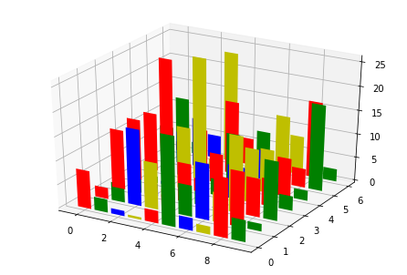

3D surface plot requires matrix processing of data:

# Create 3D figure object
fig = plt.figure()
ax = Axes3D(fig)

# Generate data
X = np.arange(-2, 2, 0.1)
Y = np.arange(-2, 2, 0.1)
X, Y = np.meshgrid(X, Y)
Z = np.sqrt(X ** 2 + Y ** 2)

# Plot surface with cmap coloring
ax.plot_surface(X, Y, Z, cmap=plt.cm.winter)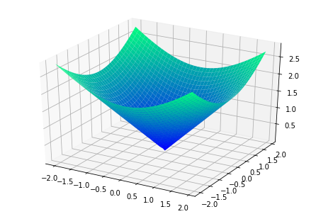

3D Mixed Plots

Mixed plots combine two different types of charts in one figure.

# Create 3D figure object
fig = plt.figure()
ax = Axes3D(fig)

# Generate data and plot figure 1
x1 = np.linspace(-3 * np.pi, 3 * np.pi, 500)
y1 = np.sin(x1)
ax.plot(x1, y1, zs=0, c='red')

# Generate data and plot figure 2
x2 = np.random.normal(0, 1, 100)
y2 = np.random.normal(0, 1, 100)
z2 = np.random.normal(0, 1, 100)
ax.scatter(x2, y2, z2)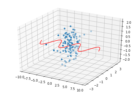

3D Subplots

We can combine 2D and 3D images together, or draw multiple 3D images together.

# Create 1 canvas
fig = plt.figure(figsize=(8, 4))

# Add subplot 1
ax1 = fig.add_subplot(1, 2, 1, projection='3d')
x = np.linspace(-6 * np.pi, 6 * np.pi, 1000)
y = np.sin(x)
z = np.cos(x)
ax1.plot(x, y, z)

# Add subplot 2
ax2 = fig.add_subplot(1, 2, 2, projection='3d')
X = np.arange(-2, 2, 0.1)
Y = np.arange(-2, 2, 0.1)
X, Y = np.meshgrid(X, Y)
Z = np.sqrt(X ** 2 + Y ** 2)
ax2.plot_surface(X, Y, Z, cmap=plt.cm.winter)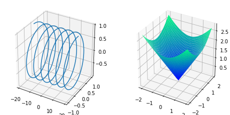

seaborn

Seaborn is built on top of Matplotlib core library with higher-level API encapsulation, allowing you to easily draw more beautiful graphics.

Quick Optimization

When using Matplotlib for plotting, the default image style is not very attractive. Seaborn can quickly optimize it.

import matplotlib.pyplot as plt
%matplotlib inline

x = [1, 3, 5, 7, 9, 11, 13, 15, 17, 19]
y_bar = [3, 4, 6, 8, 9, 10, 9, 11, 7, 8]
y_line = [2, 3, 5, 7, 8, 9, 8, 10, 6, 7]

plt.bar(x, y_bar)
plt.plot(x, y_line, '-o', color='y')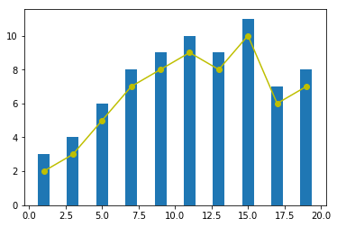

Using Seaborn for quick optimization is simple. Just place sns.set() before plotting.

import seaborn as sns

sns.set()  # Declare using Seaborn style

plt.bar(x, y_bar)
plt.plot(x, y_line, '-o', color='y')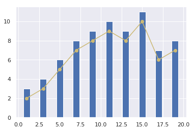

The default parameters for sns.set() are:

sns.set(context='notebook', style='darkgrid', palette='deep', font='sans-serif', font_scale=1, color_codes=False, rc=None)

Where:

context='' controls default canvas size: {paper, notebook, talk, poster}. Size: poster > talk > notebook > paper.
style='' controls default style: {darkgrid, whitegrid, dark, white, ticks}.
palette='' is the preset color palette: {deep, muted, bright, pastel, dark, colorblind}.

Seaborn Plotting API

Seaborn has about 50+ API classes. Based on application scenarios, Seaborn’s plotting methods are roughly divided into 6 categories: relational plots, categorical plots, distribution plots, regression plots, matrix plots, and combination plots.

Relational Plots

API	Description
relplot	Draw relational plot
scatterplot	Multi-dimensional scatter
lineplot	Multi-dimensional line

iris = sns.load_dataset("iris")
sns.relplot(x="sepal_length", y="sepal_width", data=iris)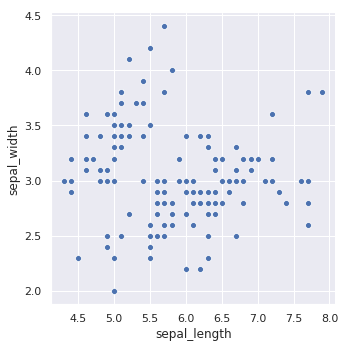

Adding category feature for coloring makes it more intuitive:

sns.relplot(x="sepal_length", y="sepal_width", hue="species", data=iris)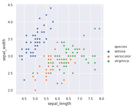

Categorical Plots

The Figure-level interface for categorical plots is catplot. It includes:

Categorical scatter: stripplot(), swarmplot()
Categorical distribution: boxplot(), violinplot(), boxenplot()
Categorical estimate: pointplot(), barplot(), countplot()

sns.catplot(x="sepal_length", y="species", data=iris)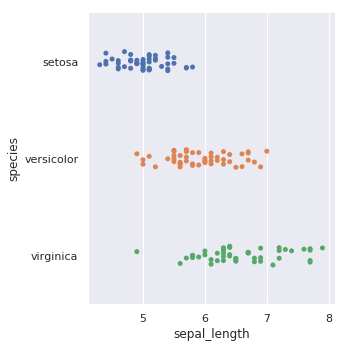

Box plot:

sns.catplot(x="sepal_length", y="species", kind="box", data=iris)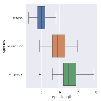

Violin plot:

sns.catplot(x="sepal_length", y="species", kind="violin", data=iris)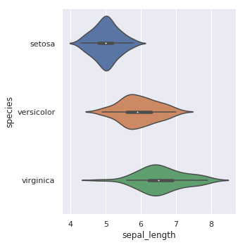

Distribution Plots

Distribution plots are used to visualize variable distributions. Seaborn provides: jointplot, pairplot, distplot, kdeplot.

sns.distplot(iris["sepal_length"])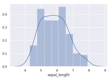

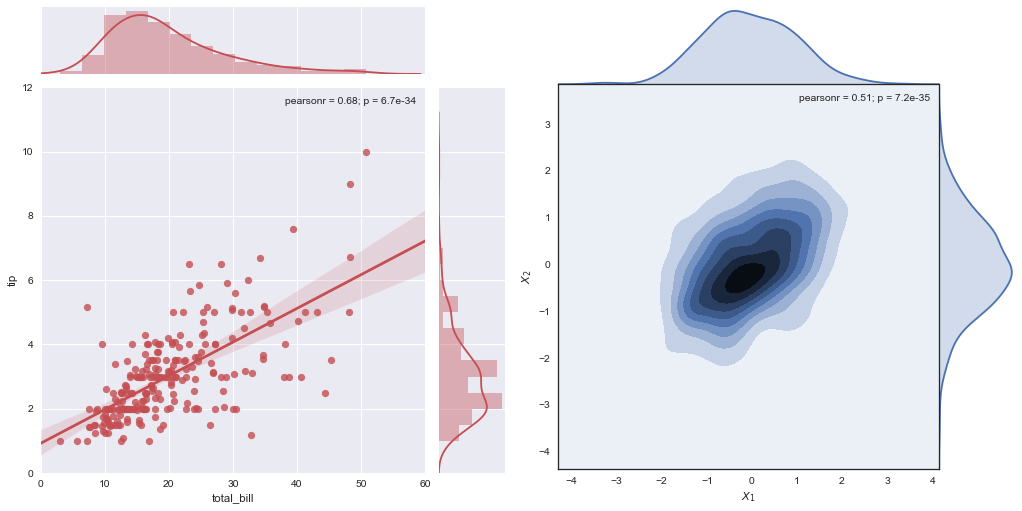
jointplot is used for bivariate distribution:

sns.jointplot(x="sepal_length", y="sepal_width", data=iris)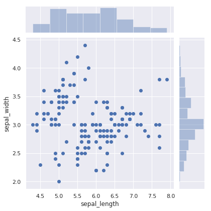

pairplot supports pairwise comparison of all features:

sns.pairplot(iris, hue="species")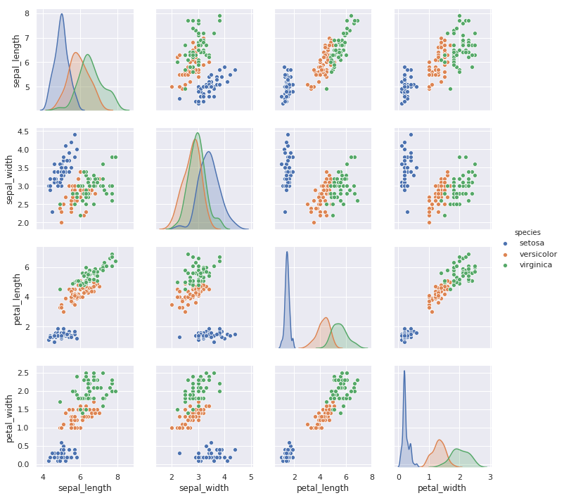

Regression Plots

Regression plot functions: lmplot and regplot.

sns.regplot(x="sepal_length", y="sepal_width", data=iris)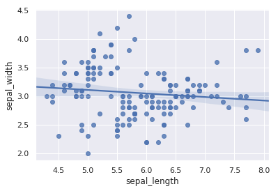

lmplot supports introducing a third dimension for comparison:

sns.lmplot(x="sepal_length", y="sepal_width", hue="species", data=iris)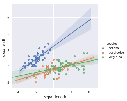

Matrix Plots

The most commonly used are heatmap and clustermap.

import numpy as np

sns.heatmap(np.random.rand(10, 10))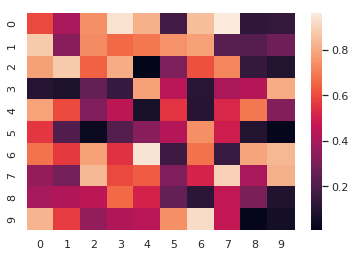

Heatmaps are very useful in certain scenarios, such as plotting variable correlation coefficient heatmaps.

Research python