As mentioned in my previous IOP paper, the mathematical essence of inversion problems is an ill-posed problem. Machine learning and deep learning essentially solve classification and regression problems, and cannot directly solve ill-posed problems. Recently, while reviewing some papers, I finally remembered some things I had read before.

Several Papers

• “Seamless retrievals of chlorophyll-a from Sentinel-2 (MSI) and Sentinel-3 (OLCI) in inland and coastal waters: A machine-learning approach”. N. Pahlevan, et al. (2020). Remote Sensing of Environment. 111604. 10.1016/j.rse.2019.111604.
• “Robust algorithm for estimating total suspended solids (TSS) in inland and nearshore coastal waters”. S.V. Balasubramanian, et al. (2020). Remote Sensing of Environment. 111768. 10.1016/j.rse.2020.111768. Code.
• “Hyperspectral retrievals of phytoplankton absorption and chlorophyll-a in inland and nearshore coastal waters”. N. Pahlevan, et al. (2021). Remote Sensing of Environment. 112200. 10.1016/j.rse.2020.112200.
• “A Chlorophyll-a Algorithm for Landsat-8 Based on Mixture Density Networks”. B. Smith, et al. (2021). Frontiers in Remote Sensing. 623678. 10.3389/frsen.2020.623678.

These papers are all by Pahlevan, with code at https://github.com/BrandonSmithJ/MDN, but they’re guarded like someone’s afraid of theft - no mention of how to reapply the methods.

Let’s look at them one by one.

Seamless retrievals of chlorophyll-a from Sentinel-2 (MSI) and Sentinel-3 (OLCI) in inland and coastal waters: A machine-learning approach

This is Pahlevan’s first paper. Let’s focus on how their network is built. The MDN principles will be explained together with the implementation later.

Training Process

Because they had enough data, they only used 1/3, about 1000 data points for training.

Input data only includes Rrs from 400-800nm.

All features are log-transformed, normalized based on median centering and interquartile scaling, and then scaled to the range (0,1).

How is this step done? I looked through their source code. For incoming data, they use from .transformers import TransformerPipeline, generate_scalers to do the transformation.

Then:

from sklearn import preprocessing
args.x_scalers = [
			serialize(preprocessing.RobustScaler),
	]
	args.y_scalers = [
		serialize(LogTransformer),
		serialize(preprocessing.MinMaxScaler, [(-1, 1)]),
	]

Wait, didn’t they say 0-1?

The specific one used should be https://scikit-learn.org/stable/modules/generated/sklearn.preprocessing.RobustScaler.html, and for y they use MinMaxScaler.

Then they should save these parameters to reuse later, otherwise where would a single number get its IQR from.

We can look at this more carefully during actual implementation.

Output data: output variables are subject to the same normalization method.

Then they put up this figure.

Wait, I don’t see where you did any feature engineering.

When reading the later papers, I noticed they removed the feature engineering part, haha. Even top journals can have issues.

Then for hyperparameter tuning:

These choices appear to be fairly robust to changes within the current implementation, especially with regard to the MDN-specific parameters. Following experimenting with several architectures, we found that the model is very robust to changes in various hyperparameters.

In this case, they only used a five-layer neural network with 100 neurons per layer, which is trained to output the parameters of five Gaussians.

The median estimates from the MDN model taken over ten trials of random network initializations are the predicted Chla for a given R**rs spectrum. Here, the same training data are used for all trials.

That’s basically it for the network part of this paper. Let’s look at the next one.

Robust algorithm for estimating total suspended solids (TSS) in inland and nearshore coastal waters

Jumping straight to the training process.

I kind of want to complain - with such direct copy-pasting, so many parts are the same, won’t this be flagged for plagiarism? The interesting thing about this paper is that it combines MDN, QAA, and water optical classification to do TSS.

The only difference from the previous paper is:

The current default model uses a five-layer neural network with 25 neurons per layer, which is trained to output the parameters of five Gaussians. From this mixture model, the overall estimate is selected via the Gaussian with the maximum prior likelihood. The described model is trained a number of times with random initializations of the underlying neural network, in order to ensure a stable final output of the estimates. The median estimate is taken as the final result of these trials, with convergence occurring within some small margin of error after approximately ten trials

Hyperspectral retrievals of phytoplankton absorption and chlorophyll-a in inland and nearshore coastal waters

No other differences.

If I had to say something, they trained two models, and I don’t quite understand why they needed two.

A Chlorophyll-a Algorithm for Landsat-8 Based on Mixture Density Networks

This one says:

All models examined in this study have simply used ‘reasonable’ default values for their hyperparameters (Glorot and Bengio 2010; Hinton 1990; Kingma and Ba 2014) namely: a five layer neural network with 100 nodes per layer, learning a mixture of five gaussians; a learning rate, L2 normalization rate, and value all set to 0.001; and with training performed via Adam optimization over a set of 10,000 stochastic mini-batch iterations, using a mini-batch size of 128 samples.

This paper is actually quite interesting.

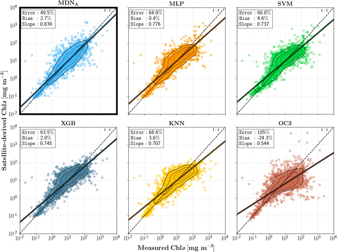
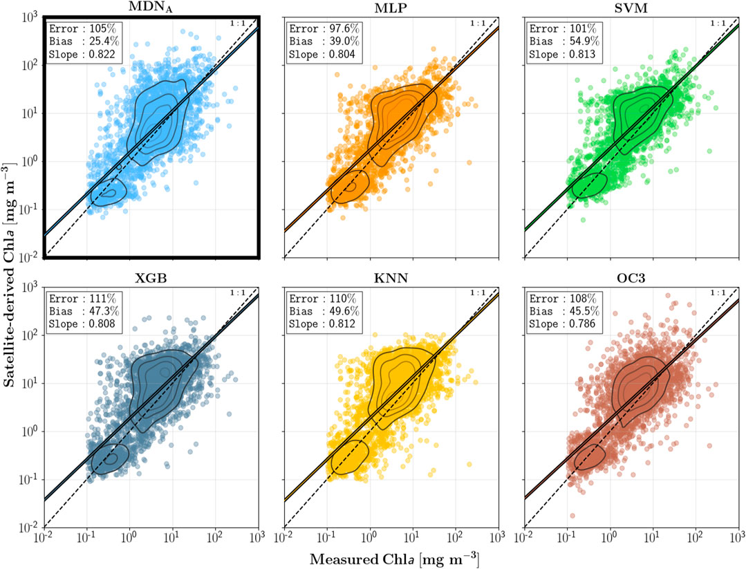
One main purpose of this paper is to demonstrate the superiority of MDN, a network architecture specifically designed for inversion problems, compared to other neural network architectures. See these figures for specific results.

They also compared XGBoost, which Cao 2020 used and I wanted to try before.

The discussion in this paper’s supplementary material is also very interesting. I feel like this discussion was written to counter a certain reviewer. Let me translate this discussion.

Reviewer asks: Why don’t you tune your model parameters?

While no hyperparameter optimization has taken place over the course of this work, it is an important step to ensure optimal performance and generality.

These choices are mostly arbitrary, as the goal of this study was to present the feasibility and theoretical backing of the MDN model

These choices are mostly arbitrary, as the goal of this study was to present the feasibility and theoretical backing of the MDN model. A full optimality demonstration, on the other hand, would require a significantly longer study than already presented.

Answer: First, that’s not the focus. Second, no time, let’s publish a paper first.

Reviewer: No, you need to prove your model parameters don’t matter.

Nevertheless, we would be remiss to exclude any discussion which examines the hyperparameter choices, and so what follows is a (very) brief look at how select parameters affect performance.

Answer: Fine, since you don’t understand, we’ll explain a bit. And we think you won’t understand anyway, so we’ll explain the simplest part.

First, some terminology must be defined in order to make it clear what is being examined. Normally in hyperparameter optimization, and machine learning in general, the dataset is split into three parts: training, validation, and testing. The training set is of course used to train the model on; the validation set is used to optimize the model using data unseen during training; and the testing set is used only at the end, in order to benchmark performance.

Answer: Let us explain the definitions for you.

As mentioned, no explicit hyperparameter optimizations have taken place thus far in the study. Default values were chosen based on those commonly used in literature and in available libraries (e.g. scikit-learn), and as will be seen, do not represent the optimal values for our specific data. As such, no separate validation set was set aside for the purposes of such an exercise.

Because we didn’t do precise hyperparameter tuning, we didn’t create a validation set, only train and test.

One of the main questions any reader may have is, “how large is the model?”.

I know you’re not in this field and can’t ask professional questions, so let me ask one.

Then they gave two figures showing the impact of layers and nodes.

Then they showed the learning curve.

Really well done roasting the reviewer, haha.

Some Knowledge Before Reading Source Code

Skip this if you don’t want to read it.

Some Knowledge About Classes

The classes I skipped before come back in another way - object-oriented programming is here again.

Classes include both variables and functions. The former are class attributes, the latter are class methods.

For example, a person’s height and weight are attributes, while speaking and eating are methods.

Definition method:

class ClassName:
   'Class help information'   # Class docstring
   class_suite  # Class body

# An example
class Employee:
   'Base class for all employees'
   empCount = 0  # Attribute

   def __init__(self, name, salary):
      self.name = name
      self.salary = salary
      Employee.empCount += 1

   def displayCount(self):  # Method
     print "Total Employee %d" % Employee.empCount

   def displayEmployee(self):
      print "Name : ", self.name,  ", Salary: ", self.salary

Here, empCount is a class variable shared among all instances, accessed via Employee.empCount.

The first method __init__() is a special method called the class constructor or initialization method. It’s called when an instance of the class is created. This means every time you create a class instance, name and salary are assigned, and Employee.empCount increments by 1.

Here, self represents the instance. For example, if you define “Li Hua”, self represents Li Hua. Think of it like defining fun(x,y,z) and calling fun(a,b,c) - self is just its internal name, you don’t need to pass it when calling.

This is a special difference between classes and functions - classes must have an extra first parameter name.

A more specific difference:

class Test:
    def prt(self):
        print(self)
        print(self.__class__)
t = Test()
t.prt()

Output:

<__main__.Test instance at 0x10d066878>
__main__.Test

The first line outputs instance, representing an instance. The second line is the class itself.

self is not a keyword - you could change it to akb48.

To call, you must create an instance:

# "Create first Employee object"
emp1 = Employee("Zara", 2000)
# "Create second Employee object"
emp2 = Employee("Manni", 5000)

These parameters are received through init.

Similar to functions, you can modify and access attributes within instances:

emp1.displayEmployee()
emp2.displayEmployee()
print "Total Employee %d" % Employee.empCount

Output:

Name :  Zara ,Salary:  2000
Name :  Manni ,Salary:  5000
Total Employee 2

You can also add, delete, and modify class attributes:

emp1.age = 7  # Add 'age' attribute
emp1.age = 8  # Modify 'age' attribute
del emp1.age  # Delete 'age' attribute

You can also use these functions to access attributes:

• getattr(obj, name[, default]): Access object attribute
• hasattr(obj, name): Check if attribute exists
• setattr(obj, name, value): Set attribute. Creates new if doesn’t exist
• delattr(obj, name): Delete attribute

hasattr(emp1, 'age')    # Returns True if 'age' exists
getattr(emp1, 'age')    # Returns value of 'age'
setattr(emp1, 'age', 8) # Add attribute 'age' with value 8
delattr(emp1, 'age')    # Delete attribute 'age'

Python has some built-in class attributes that exist when you create a class:

• dict: Class attributes (dictionary of class data attributes)
• doc: Class docstring
• name: Class name
• module: Module where class is defined
• bases: All parent classes (tuple of parent classes)

Access method:

class Employee:
   'Base class for all employees'
   empCount = 0

   def __init__(self, name, salary):
      self.name = name
      self.salary = salary
      Employee.empCount += 1

   def displayCount(self):
     print "Total Employee %d" % Employee.empCount

   def displayEmployee(self):
      print "Name : ", self.name,  ", Salary: ", self.salary

print "Employee.__doc__:", Employee.__doc__
print "Employee.__name__:", Employee.__name__
print "Employee.__module__:", Employee.__module__
print "Employee.__bases__:", Employee.__bases__
print "Employee.__dict__:", Employee.__dict__

Output:

Employee.__doc__: Base class for all employees
Employee.__name__: Employee
Employee.__module__: __main__
Employee.__bases__: ()
Employee.__dict__: {'__module__': '__main__', 'displayCount': <function displayCount at 0x10a939c80>, 'empCount': 0, 'displayEmployee': <function displayEmployee at 0x10a93caa0>, '__doc__': '\xe6\x89\x80\xe6\x9c\x89\xe5\x91\x98\xe5\xb7\xa5\xe7\x9a\x84\xe5\x9f\xba\xe7\xb1\xbb', '__init__': <function __init__ at 0x10a939578>}

Class Inheritance and Polymorphism

The biggest benefit of object-oriented programming is code reuse.

Code is easier to understand:

class Parent:        # Define parent class
   parentAttr = 100
   def __init__(self):
      print "Calling parent constructor"

   def parentMethod(self):
      print 'Calling parent method'

   def setAttr(self, attr):
      Parent.parentAttr = attr

   def getAttr(self):
      print "Parent attribute :", Parent.parentAttr

class Child(Parent): # Define child class
    # class DerivedClassName(BaseClassName)
   def __init__(self):
      print "Calling child constructor"

   def childMethod(self):
      print 'Calling child method'

c = Child()          # Instantiate child class
c.childMethod()      # Call child method
c.parentMethod()     # Call parent method
c.setAttr(200)       # Call parent method again
c.getAttr()          # Call parent method again

Parent classes only define the most basic attributes and methods.

Polymorphism is like adding this method to Employee:

class Employee:
   'Base class for all employees'
   empCount = 0

   def __init__(self, name, salary):
      self.name = name
      self.salary = salary
      Employee.empCount += 1

   def displayCount(self):
     print "Total Employee %d" % Employee.empCount
   def print_title(self):
        if self.sex == "male":
            print("man")
        elif self.sex == "female":
            print("woman")

   def displayEmployee(self):
      print "Name : ", self.name,  ", Salary: ", self.salary

Now if we want to hire child workers, we can write a new subclass:

class child(Employee):
     def print_title(self):
        if self.sex == "male":
             print("boy")
         elif self.sex == "female":
             print("girl")

When both child and parent have the same print_title() method, the child’s print_title() overrides the parent’s. At runtime, the child’s print_title() is called.

The benefit of polymorphism is that when we need more subclasses like Teenagers, Grownups, etc., we just inherit from Person. The print_title() method can either not be overridden (use Person’s) or be overridden with a specific one. This is the “Open-Closed” principle.

Iterator

About what kind of class can be looped - I feel I don’t need this for now.

Access Restriction

If we don’t want an attribute to be accessed externally, we can add access restrictions:

class JustCounter:
	__secretCount = 0  # Private variable
	publicCount = 0    # Public variable

	def count(self):
		self.__secretCount += 1
		self.publicCount += 1
		print self.__secretCount

counter = JustCounter()
counter.count()
counter.count()
print counter.publicCount
print counter.__secretCount  # Error, instance cannot access private variable

Module Import

A Python module is a Python file ending in .py, containing Python object definitions and statements.

This means we can put classes in modules and call them like functions.

MDN Implementation

After all that, what is MDN?

I plan to explain it together with this.

Let’s focus on how they implement MDN, then compare with the paper’s source code. Finally, we’ll explain the principles.

Before reading this, please complete this tutorial first.

class MDN(nn.Module):
    def __init__(self, n_hidden, n_gaussians):
        super(MDN, self).__init__()
        self.z_h = nn.Sequential(  # Sequential processing: linear transformation then tanh
            nn.Linear(1, n_hidden),  # Linear transformation here
            nn.Tanh()
        )
        self.z_pi = nn.Linear(n_hidden, n_gaussians)
        self.z_sigma = nn.Linear(n_hidden, n_gaussians)
        self.z_mu = nn.Linear(n_hidden, n_gaussians)
    def forward(self, x):
        z_h = self.z_h(x)
        pi = nn.functional.softmax(self.z_pi(z_h), -1)
        # rescale to [0,1]
        sigma = torch.exp(self.z_sigma(z_h))
        # exp operation
        mu = self.z_mu(z_h)
        return pi, sigma, mu

Let’s explain in detail how this MDN is constructed.

For each input x, we predict the distribution of y:

$P(y|x) = \sum_{k}^{K} \Pi_{k}(x) \phi(y, \mu_{k}(x), \sigma_{k}(x))$

• $k$ is an index describing which Gaussian we are referencing. There are $K$ Gaussians total.
• $\sum_{k}^{K}$ is the summation operator. We sum every $k$ Gaussian across all $K$. You might also see $\sum_{k=0}^{K-1}$ or $\sum_{k=1}^{K}$ depending on whether an author is using zero-based numbering or not.
• $\Pi_k$ acts as a weight, or multiplier, for mixing every $k$ Gaussian. It is a function of the input $x$: $\Pi_k(x)$
• $\phi$ is the Gaussian function and returns the at $y$ for a given mean and standard deviation.
• $\mu_k$ and $\sigma_k$ are the parameters for the $k$ Gaussian: mean $\mu_k$ and standard deviation $\sigma_k$. Instead of being fixed for each Gaussian, they are also functions of the input $x$: $\mu_k(x)$ and $\sigma_k(x)$

All of $\sigma_{k}$ are positive, and all of the weights $\Pi$ sum to one:

$\sum_{k}^{K} \Pi_{k} = 1$

First our network must learn the functions $\Pi_{k}(x), \mu_{k}(x), \sigma_{k}(x)$ for every $k$ Gaussian. Then these functions can be used to generate individual parameters $\mu_k, \sigma_k, \Pi_k$ for a given input $x$. These parameters will be used to generate our pdf $P(y|x)$. Finally, to make a prediction, we will need to sample (pick a value) from this pdf.

In our implementation, we will use a neural network of one hidden layer with 20 nodes. This will feed into another layer that generates the parameters for 5 mixtures: with 3 parameters $\Pi_k$, $\mu_k$, $\sigma_k$ for each Gaussian $k$.

Our definition will be split into three parts.

First we will compute 20 hidden values $z_h$ from our input $x$.

$z_h(x) = \tanh( W_{in} x + b_{in})$

Second, we will use these hidden values $z_h$ to compute our three sets of parameters $\Pi, \sigma, \mu$:

$z_\Pi = W_{\Pi} z_h + b_{\Pi}\\ z_\sigma = W_{\sigma} z_h + b_{\sigma}\\ z_\mu = W_{\mu} z_h + b_{\mu}$

Third, we will use the output of these layers to determine the parameters of the Gaussians.

$\Pi = \frac{\exp(z_{\Pi})}{\sum_{k}^{K} \exp(z_{\Pi_k})}\\ \sigma = \exp(z_{\sigma})\\ \mu = z_{\mu}$

• $\exp(x)$ is the exponential function also written as $e^x$

We use a softmax operator to ensure that $\Pi$ sums to one across all $k$, and the exponential function ensures that each weight $\Pi_k$ is positive. We also use the exponential function to ensure that every $\sigma_k$ is positive.

I understand now - the way this is constructed is that MDN predicts several parameters of a Gaussian Mixture Model, then takes values from the entire PDF as predictions.

This leads to a question: my y value is only one number, but MDN produces a distribution. How do we calculate loss to update weights?

See the next article.